We’re delighted to once again have Mark Laceky, President of mLogic Consulting as guest blogger. mLogic’s previous post explained one of their favorite measures, Base Weighted Weeks (BWW). This follow-up post gives a concrete example of how to use BWW and includes an Excel-based tool that you can download and use yourself.

Keep in mind that this post falls into the “Advanced” category! If you are fairly new to the CPG industry and/or to syndicated POS data, then you may want to check out some of our other posts. If you have any questions on this specific post or the Excel file, PLEASE contact mLogic directly via email at info@mlogicconsulting.com. And now, on with the show!
The Only Constant Is Change
As any Marketer and Analyst can tell you, plans change. They change all the time. And the people who change them want to know (yesterday) what the sales impacts are likely to be based on those changes. Or worse – they have 18 ideas about changes they might want to make and they want someone (you) to estimate the impacts of each. What if we raise price and spend back? What if our trade budgets get cut 20%? What if we add a feature week? What if we promote with deeper discounts? How much would it drive sales if we got more displays?
If you’re the person responsible for providing answers/estimates on the fly you’ve probably devised some sort of spreadsheet to help you do the calculations, right? It has some syndicated POS data in it (baselines and base prices? incremental volumes and promoted prices? current distribution? category trend?). And then there are all those other business drivers that you can’t get from your syndicated POS Nielsen or IRI database – consumer promotion, advertising, package changes, etc. Of course, there are also lots of assumptions that make the whole thing work, right?
We can’t help you estimate the impact of changes to all of the drivers, but we can help you with the price and promotion end of things – using data that is available in your Nielsen or IRI database. (Note: If the mention of business drivers sounds familiar, you may have read about them in the series of posts on Volume Decomposition in the CPG Data Tip Sheet. This first of the 6 posts gives an overview of how to attribute past sales to the various business drivers and Part 6 talks about the “other drivers.” While a volume decomp analysis looks backwards to explain what happened, the methodology and tool in this post looks into the future to estimate what is likely to happen using similar concepts.)
Bringing It All Together – A Unified Approach To Estimating Sales Impacts
Our previous article reviewed Base Weighted Weeks (BWW) as a better measure of promotion frequency with the added benefit that all the math works out to the last decimal point. This article (and the attached “prize inside”) will show you how to use BWW and some other concepts together to create a simple but powerful sales estimation tool to make your life easier (part of it anyway). CAVEAT: this approach is recommended only when you don’t have more powerful tools on hand (such as price/promotion models, marketing mix models, etc).
CLICK HERE to download the pre-built Excel tool that we call Impact Estimator. It gets you from data pull to simulator and does all the math for you. Of course, if you’re curious about the formulas you can explore the tool. But for lighter reading, here are the key concepts:
- There is a standard POS data pull template you should start using (1. Data Pull tab)
- It has everything in it so you don’t have to keep going back to the well – pull data just once!
- Link all calculations in the other 2 tabs to this raw data pull to build your Impact Estimator
- Break all business driver inputs into individual pieces that are multiplicative! That is, turn each individual component into an impact index, then multiply all the indices together to get the net impact.
- Start with baseline volume drivers then move to incremental volume drivers.
- Baseline volume drivers are anything not related to in-store trade promotions. Base drivers include base price changes, distribution changes, changes to advertising, changes to consumer promotion, category trends, changes in competitive impacts, etc.
- You’re on your own estimating some of these impacts – the secret is to estimate them one by one. You can go back later and change your assumptions if you like.
- Example: category is growing at 4% so our brand will likely grow at 4% or an index of 1.04.
- There are three incremental volume drivers – promotion frequencies, mix by promotion type and discount levels. The tool automatically fills in the current BWWs and discounts for each of the mutually exclusive and additive promotion types and the user then inputs changes:
- TPR (a temporary price reduction with no ad and no display present)
- Feature Ad w/o Display (a feature ad with no display present)
- Display w/o Feature Ad (a display with no feature ad present)
- Feature & Display (a feature ad with a display present)
- The Impact Estimator tool automatically calculates a Promoted Price Elasticity (PPE) based on the % lift and % discount on TPRs and then calculates multipliers for ads and displays. The user then can input new promoted discounts and watch volumes change accordingly
Example: Geography A, Brand X, Category Z, 1-Year
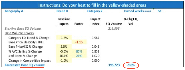
Note that the tables shown below are all in the Simulator tab in the Impact Estimator Excel tool. Starting with Baseline Volume Drivers, the user enters inputs into yellow-shaded cells (rows 9-14):

In this example, we are assuming the category volume trend will be -1.3%, Brand X base price/EQ will go up +5.0%, % ACV Distribution will drop 5% (not points), average items carried will be up +10% and competitors will be doing something (trade promotion? distribution gain? advertising?) that will cause Brand X to lose 1% of its volume.
As noted in the tool, there are some assumptions being made:
- Base Price Elasticity (BPE) is a simple estimate of ¾ of the Promoted Price Elasticity (PPE) – this is a general rule of thumb. If you have a BPE from previous research use that instead.
- For % ACV Distribution we are assuming an 85% incrementality rule – that is, if we get 5% less distribution we’ll only see a 4.25% loss in volume (due to reduced cross-store cannibalization and assuming that stores that drop distribution don’t sell as fast anyway).
- For average items carried we’re assuming a 20% incrementality rule. That is, getting 10% more items on shelf (e.g. going from 10 to 11 where carried) will only increase volume by 2% due to the new item being a slower mover and cannibalizing from existing items on shelf.
The net result is a Baseline Volume % Change estimate of -9.8% (in cell I15).
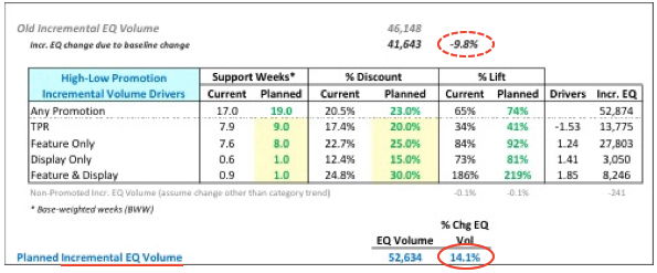
Then we move on to the Incremental Volume (Rows 23-26). The starting rule is that (with no changes to the trade promotion plan) incremental volume would be down the same % as base volume (in this case -9.8%). Then we move to changing the trade promotion plan:

In this example, we’ve increased total promotion frequency from 17.0 BWW to 19.0 BWW by increasing the frequency of each of the four promotion types. We also increased the discount levels slightly for each promotion type. The result is that our incremental volume should go up by +14.1% (cell I30) instead of being down -9.8% due to the baseline dropping.
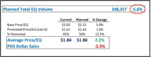
The net result (rows 32-39) of all the changes is that Total EQ Volume should drop -5.6%. And since the Average Price/EQ will only be up 2.2%, we would expect our dollar sales to be down -3.5%.

The Upshot?
This article and tool are meant to be useful by highlighting some key concepts and then bringing them all to bear inside a unified approach. Key ideas are:
- The right data pull means you only have to do it once
- Always handle base drivers separately from incremental drivers
- Break all of your assumptions into manageable, multiplicative pieces
- Promotion changes are very manageable using BWW, PPE and multipliers – which in turn are easy to glean from the data
We hope some or all of these concepts make it into your own sales estimation tool!
Please direct comments and questions about this article directly to Mark. His contact details are below.
Mark Laceky is President and founder of mLogic Consulting, Inc. which specializes in consumer packaged goods (CPG) pricing and trade promotion strategy. He previously managed the Nielsen North America Price & Promotion analytics practice and spent years in analytical leadership roles at Kraft Foods and The Quaker Oats Company. He may be reached via LinkedIn or by email at info@mlogicconsuting.com.

Hello,
Is there any aspect of merchandizing (supports or pricing) that can influence baseline volumes?
Ideally supports and merch price would be incremental drivers; but keen to know if any aspect of merch can influence my baseline volumes?
Mark Laceky replies:
The short answer to this question begins with a reminder of the technical definition of what a baseline is and what it isn’t. Baselines are simply estimates at the UPC-level of what unit sales would have been in a store in a week when there was some form of in-store merchandising as recognized by Nielsen or IRI. These forms of direct-item merchandising only include TPR’s (typically at least a 7% discount), feature ads (circulars, newspapers, etc) or displays (temporary, secondary placement in the store).
Everything else that happens can have an impact on baselines. Some examples:
a) All other forms of in-store merchandising (Shelf Talk, floor ads, Catalina coupons, sampling, long-term displays, spend $20/get $5″, etc)
b) All advertising or consumer promotion (FSI’s, sweepstakes, radio, tv, internet ads, online ads, etc)
c) Many others factors including seasonality, weather, store closings, competitive actions, distribution changes, price changes, shelf set changes, etc
Finally, there is a technical issue that some of you may have noticed – “Why is it that some of my baselines spike whenever there is a trade promotion?”. There are a few possible answers but two of them likely explain most cases.
d) First are FSI’s run at the same time as an in-store promotion – if your baseline is “cross-sectionally adjusted” (that is, the algorithm looks across all stores in a market in a given week) then an FSI will cause a baseline spike, even in stores that promoted.
e) Second are “slow-movers” – some UPC’s sell zero units in some stores in some weeks when not promoted but will sell some units during a promotion. The baseline during the weeks when there are zero units will be zero but in the week of the promotion the baselines for these UPCs will jump to at least 1 unit. So when you’re looking at a PPG or any other aggregate of UPCs during a promotion the baseline for that subtotal will include some baseline spikes for the slow-moving UPCs in that aggregate.
Here’s a question from reader Ben S.:
“First, thank for putting this together. It has some very helpful ideas! But I have a real problem with the data pull that renders it almost unusable. Not sure HOW to get the data to pull the way it is put together using IRI Advantage.” Ben then goes on to describe why it is difficult to pull the facts in the same order that Mark has them in his Excel file. Although it is straightforward to pull the facts from Nielsen in the order that Mark has, it is not so simple in IRI. This is because in IRI they treat the merchandising condition (Non-Promoted, Feature, Display, Feat & Disp and TPR) as a 5th dimension so that all facts related to a condition are all next to each other in the data pull. (Note: if you are not an IRI user, no need to worry about this.)
Here is Mark’s reply:
You can either research how to reorder the facts in IRI Advantage or simply reorder (via cut and paste) the order of the rows in the Data Pull tab to match whatever order your IRI data pull is in. If you re-order the rows in the Data Pull sheet via cut and paste the other two sheets in the file will not need changing.
In the factor column of the Impact investigator, we have Elasticity, and factors on ACV and # of items change.
I know that elasticity is, but the factor for the other two – can someone help me understand what’s behind these two numbers?
Thanks.
I assume you are asking about the numbers in cells F12 and F13 in the Excel file. These are assumptions made as to the elasticity of the 2 components of distribution. There are specific analyses that can be done to derive these types of elasticities. As Mark says in the post:
– For ACV, we are assuming an 85% incrementality rule – that is, if we get 5% less distribution we’ll only see a 4.25% loss in volume (due to reduced cross-store cannibalization and assuming that stores that drop distribution don’t sell as fast anyway).
– For average items carried we’re assuming a 20% incrementality rule. That is, getting 10% more items on shelf (e.g. going from 10 to 11 where carried) will only increase volume by 2% due to the new item being a slower mover and cannibalizing from existing items on shelf.
If you have any further questions, feel free to contact Mark directly.
Thank you very much for explaining this! It seems so obvious now.